Convolution

---

As anticipated in the article “Toolbox for studying DSP”, a signal is an object that carries information about the variation of one variable with respect to another reference. In the case of audio signals: how the sound amplitude varies with respect to time.

Signals can be of infinitely many types, but there are some well-known, simple, and particularly recurring ones. For now, let’s focus on one in particular: the Dirac impulse \(δ(t)\). It is a signal that is \(=0\) at all instants except at a single point, where ideally it is infinite. From a sound perspective, we could imagine it as a very loud click in amplitude and very short in time.

Let’s imagine being in a large empty room and emitting this click through a speaker. What happens? Initially, our ears will be reached by the direct signal emitted by the speaker. Shortly after, the primary reflections will arrive, and later a tail of secondary reflections. We can imagine the situation more or less like this:

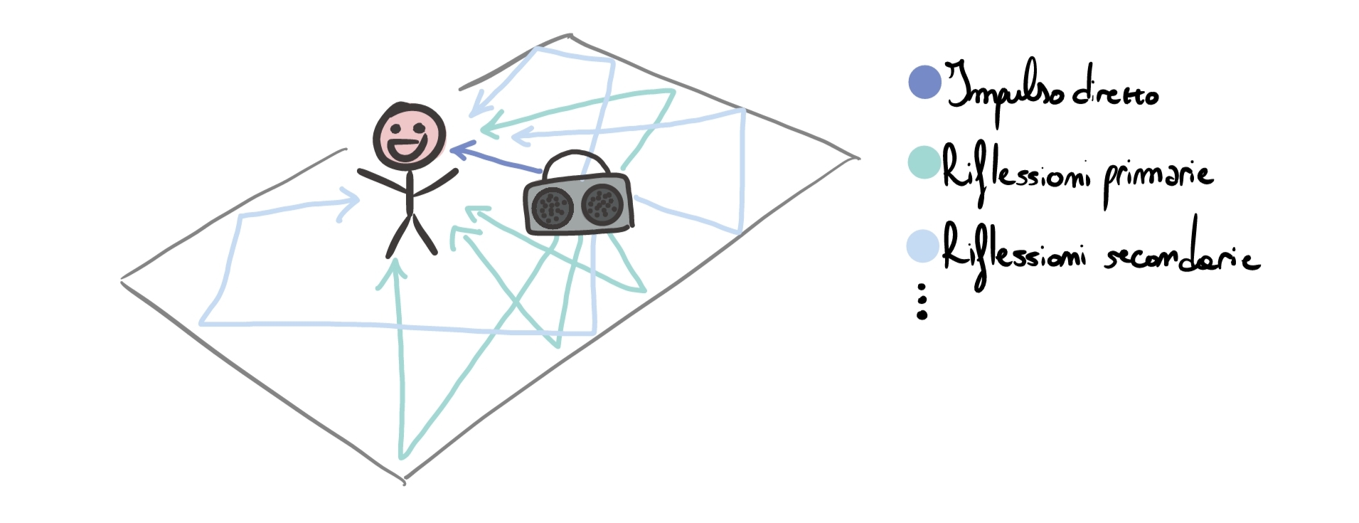
Let’s imagine placing a microphone where the listener is (for the moment we ignore directivity, attenuation, and any other complication) and recording the result of emitting the impulse in the room: we will obtain an audio file representing the direct impulse plus the various reflections. This recording is called the Impulse Response and it is the fingerprint of the “room” system. It is then possible to use the IR \(=h(t)\) to emulate the room, like this:

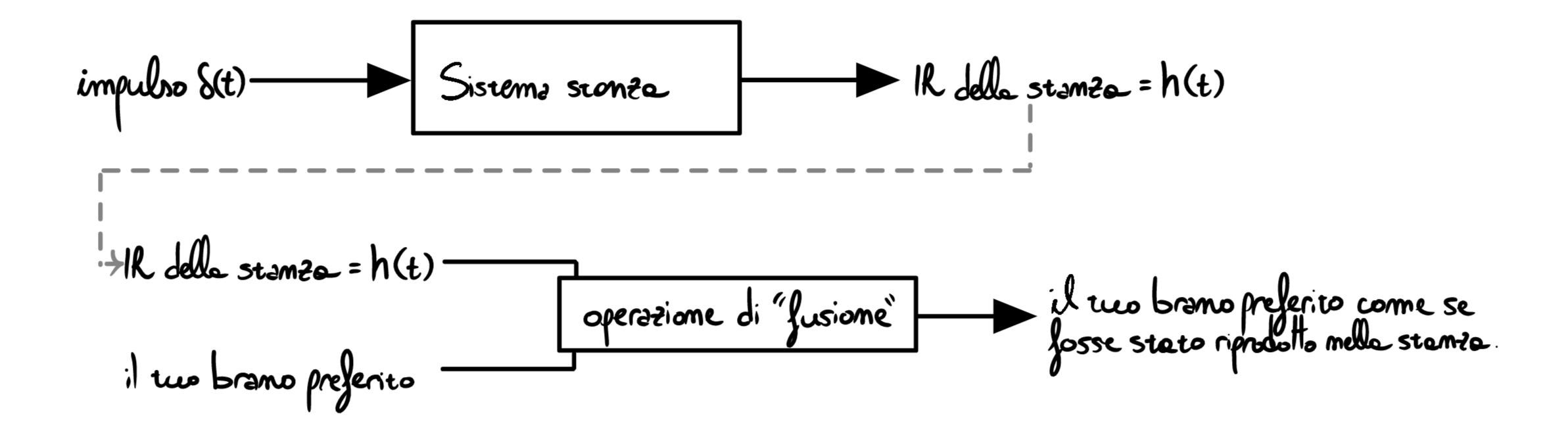
The blending operation in the image above is the topic that will guide the rest of the article: convolution.

Convolution

Let’s imagine we want to apply the Impulse Response obtained from the previous recording to a single hand clap \(x(t)\).

Let’s think carefully about the differences between the original signal \(x(t)\) and the modified one \(y(t)\) that we want to obtain:

• \(x(t)\) contains the single clap, then silence.
• \(y(t)\) contains the same clap, and then the reverberations, that is repetitions of the initial clap, delayed in time and attenuated in amplitude, which create “the illusion that the clap was produced in the room”.

In practice, \(y(t)\) is the result of applying a law that transforms the signal \(x(t)\) into a new \(y(t)\) by combining past and present samples of the original signal. In “math language”, in the discrete domain: \(y[n]=\sum_{k=-\infty}^{+\infty} x[k]\cdot h[n-k]\), where \(h\) is precisely the IR (the filter) we are applying. The operation described by the previous formula is called convolution and is indicated with the symbol \(*\).

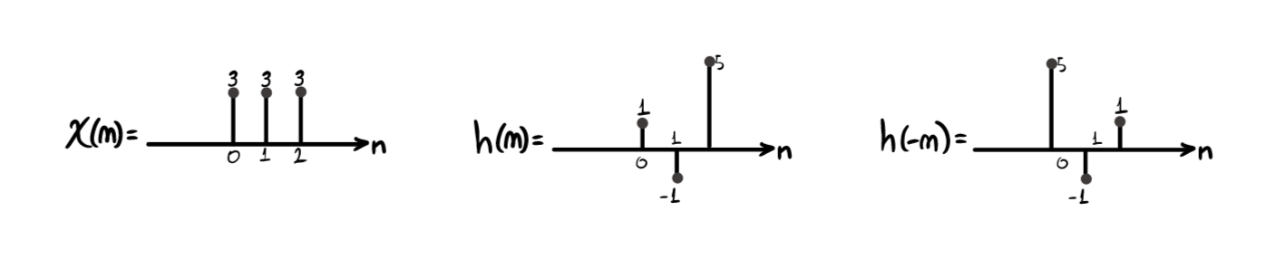
Computing the convolution \(y[n]=x[n]*h[n]\) of two signals is boring, long, repetitive, and costly, but also conceptually simple. Consider for example:

• the signal \(x(n)=3\delta[n]+3\delta[n-1]+3\delta[n-2]\)
• a filter \(h(n) = \delta[n]-1\delta[n-1]+5\delta[n-2]\)

the filtering can be performed through the following algorithm:

• “Flip” \(h(n)\), obtaining \(h(-n)\).

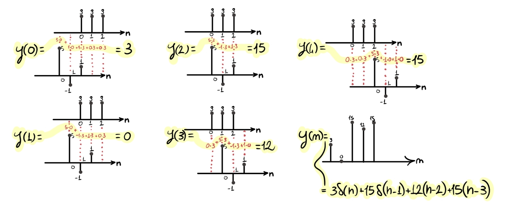
• “Take” \(h(-n)\) and, for every possible position, shift it from left (\(-\infty\)) to right (\(+\infty\)), performing the sample-by-sample multiplication between \(x(n)\) and \(h(n)\). Then, sum the partial results obtained (obviously, it is not necessary to really start from \(-\infty\); it is enough to start from the first position where \(x(n)\) and \(h(-n)\) have an overlapping sample). Each of these shifts will return one sample of the new output signal \(y(n)\), the result of the convolution.

Convolution carried out this way is very expensive in terms of computational resources, so it is absolutely not suitable for low-power environments or systems that must work in real time. We will see the solution to this problem in a later chapter.

This operation has interesting properties. The ones that, in my opinion, are worth remembering for “everyday use” are: commutativity, associativity, linearity, time invariance.

This last property, in particular, will serve as a transition between this topic and the next one.

LTI systems, complex exponential, and the frequency domain

(Simplifying) a system \(T\) that, given an input \(x[n]\), produces an output \(y[n]=T\{x[n]\}\), is time-invariant if a time shift of the input results only in the same time shift of the output, that is if \(T\{x[n-n_0]\} = y[n-n_0]\).

A system is linear if it does not introduce nonlinearities in the output, that is if the following two principles hold:

• Additivity: the response to a sum is the sum of the responses. -> \(T\{x_1[n]+x_2[n]\}=T\{x_1[n]\}+T\{x_2[n]\}\)
• Scalability: the response to a scaled signal is scaled in the same way. -> \(T\{\alpha x[n]\}=\alpha\,T\{x[n]\}\)

Obviously, a Linear Time-Invariant (LTI) system enjoys all the properties just mentioned: \(y[n] = (h*x)[n] = \sum_{k=-\infty}^{\infty} h[k]\;x[n-k]\).

Now, consider the complex exponential \(e^{j\omega n}\), which by Euler’s identity seen in this article is equal to the sum of sinusoids \(e^{j\omega n}=\cos(\omega n)+j\sin(\omega n)\).

Take an LTI system with impulse response \(h[n]\). We have seen that its output can be computed through convolution \(y[n]=\sum_{k=-\infty}^{+\infty} h[k]\;x[n-k]\). Setting the input to \(x[n]=e^{j\omega n}\) and substituting into the formula, we obtain:

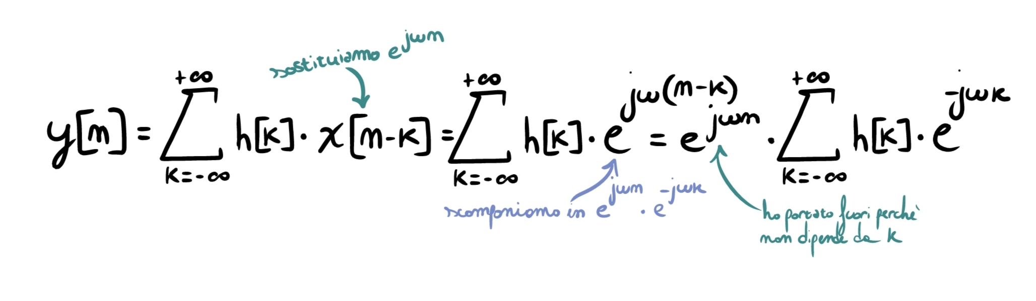
As you can see, the term \(\sum_{k=-\infty}^{+\infty} h[k]\,e^{-j\omega k}\) does not depend on time \(n\) in any way, but only on the filter (\(k\)). We define this quantity as \(H(e^{j\omega})=\sum_{k=-\infty}^{+\infty} h[k]\,e^{-j\omega k}\): it is the frequency response of the system, that is, the response of the system when it receives pure sinusoids at frequency \(\omega\) as input (in this case, we provided \(e^{j\omega n}=\cos(\omega n)+j\sin(\omega n)\)). From now on, we will work a lot with this concept.

Going back to the current case, we can therefore rewrite the equation as \(y[n]=e^{j\omega n}\,H(e^{j\omega})\). We notice several important things:

• the shape of the output signal is still \(e^{j\omega n}\);
• the system does not create new frequencies;
• all it does is multiply the signal by a complex number.

For this reason, \(e^{j\omega n}\) is said to be an eigenfunction of LTI systems.

I understand that all of this may look like an absurd complication without a precise purpose, but we will see that it is not.

My buddy Fourier

Up to this point we have seen that an LTI system has a fundamental property: if we feed a complex exponential \(e^{j\omega n}\) at the input, we obtain the same shape at the output, multiplied by a complex number \(H(e^{j\omega})\).

This observation alone is not enough. The natural question is: why should this help us describe real signals, which are not complex exponentials at all?

A real signal is not a single sinusoid, it does not have a single frequency, and it varies over time in a complex way. However, there is a fundamental fact: any signal can be seen as the sum of many elementary components, each oscillating at its own frequency. These elementary components are precisely the complex exponentials \(e^{j\omega n}\).

In other words, instead of describing a signal in time as “a complicated shape”, we can describe it as a collection of frequencies, each with a certain amplitude and a certain phase. This is the idea behind Fourier representation.

If we also assume we are working with LTI systems, the superposition principle holds:

• the response to a sum is the sum of the responses
• the response to a scaled signal is scaled in the same way

This means something very powerful: if I know the system’s response to each elementary component, I know the response to the complete signal.

If a signal is the sum of many sinusoids, and the system responds to each sinusoid by multiplying it by \(H(e^{j\omega})\), then the output will simply be the sum of all these modified sinusoids. There is no need to do anything “extra”.

If in the time domain filtering required a convolution: \(y[n]=\sum_{k=-\infty}^{+\infty} h[k]\;x[n-k]\) (very expensive), in the frequency domain each frequency component of the signal is treated independently, being simply multiplied by a complex number.

Let’s anticipate the result: convolving in time corresponds to multiplying in frequency.

Why is this useful? Simply because multiplying is infinitely less expensive than convolving. This is why we often analyze systems in the frequency domain, design filters by looking at \(H(e^{j\omega})\), and use Fourier and FFT (which we will see shortly) in real audio processing.

Fourier series

For now, let’s restrict ourselves to the case of periodic discrete signals. In particular, consider a periodic discrete signal \(x[n]\) with period \(N\): \(x[n] = x[n+N]\).

This constraint has a fundamental consequence: the frequencies that compose it must also be periodic, and therefore can assume only specific values.

In the discrete domain, the only complex exponentials compatible with periodicity \(N\) are those for which \(e^{j\omega (n+N)} = e^{j\omega n}\):

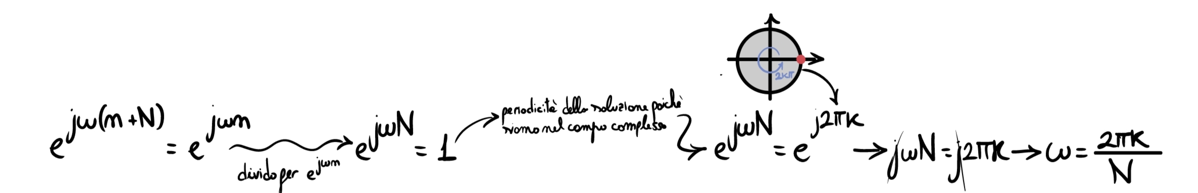
so the allowed frequencies are not continuous, but discrete.

Given all this, a periodic signal \(x[n]\) can be written through the discrete Fourier Series \(x[n] = \sum_{k=0}^{N-1} X[k]\;e^{j\frac{2\pi}{N}kn}\), where:

• \(e^{j\frac{2\pi}{N}kn}\) are the basic sinusoidal components;
• \(X[k]\) are complex coefficients;
• \(N\) is the signal period.

This formula says that the time-domain signal is a linear combination of sinusoids at frequencies that are multiples of the fundamental \(\frac{2\pi}{N}\). The coefficients \(X[k]\) in the formula are obtained through: \(X[k] = \frac{1}{N}\sum_{n=0}^{N-1} x[n]\;e^{-j\frac{2\pi}{N}kn}\).

You do not need to memorize this formula now: it is only needed to understand that each coefficient measures “how much” of that frequency is present and that the signal is completely described by the set of \(X[k]\).

Physically, each term of the sum \(X[k]\;e^{j\frac{2\pi}{N}kn}\) represents a sinusoid with angular frequency \(\omega_k = \frac{2\pi}{N}k\), amplitude \(\|X[k]\|\), and phase \(\angle X[k]\). In the frequency domain, each k corresponds to a spectral line, so the spectrum is a discrete sequence of impulses.

Fourier transform

The Fourier Series allowed us to describe periodic discrete signals as a sum of sinusoids at discrete frequencies. However, most real signals are not periodic: a spoken word, a snare hit, a hand clap, or any isolated sound event does not repeat identically over time.

So what happens if we remove the periodicity constraint?

When a signal is not periodic, there is no longer a period N that imposes a grid on the allowed frequencies and, consequently, the spectrum is no longer made of discrete lines, but becomes continuous. In this case, the representation of the signal in the frequency domain is provided by the Discrete-Time Fourier Transform: \(X(e^{j\omega}) = \sum_{n=-\infty}^{\infty} x[n]\;e^{-j\omega n}\).

Conceptually:

• \(x[n]\) describes what happens in time;
• \(X(e^{j\omega})\) describes how much energy is present at each frequency and with which phase.

Also in this case, \(X(e^{j\omega})\) is a complex quantity. Its magnitude \(\|X(e^{j\omega})\|\) indicates the amplitude of the frequency components, while its argument \(\angle X(e^{j\omega})\) indicates the phase.

Unlike the Fourier Series, here \(\omega\) varies continuously. This means that the spectrum is no longer a sequence of lines, but a continuous function of frequency.

Note that going from the time domain to the frequency domain involves a trade-off: in the time domain we know when events happen, in frequency we know which frequencies they are made of. This means that the Fourier Transform provides a global description of the signal: it tells which frequencies are present and with what weight, but it does not preserve precise time information. We no longer know at which instant a certain component appeared, only that it is present in the overall signal.

So there are cases where it is better to work in time, and cases where it is convenient to move to frequency.

Convolution and multiplication: the fundamental property

At this point we have introduced two concepts that seem to live in different worlds:

• in the time domain, an LTI system filters through convolution;
• in the frequency domain, a signal is described by its spectrum \(X(e^{j\omega})\).

The central point of the article is that these two worlds are linked by an extremely powerful property:

\[y[n] = x[n] * h[n] \quad \Longleftrightarrow \quad Y(e^{j\omega}) = X(e^{j\omega}) \cdot H(e^{j\omega})\]

Read it like this: if in time the output is the convolution between input \(x[n]\) and impulse response \(h[n]\), then in frequency the output spectrum \(Y(e^{j\omega})\) is obtained simply by multiplying the input spectrum \(X(e^{j\omega})\) by the filter’s frequency response \(H(e^{j\omega})\).

In practice, filtering a signal means “shaping” its frequency content: \(Y(e^{j\omega}) = X(e^{j\omega}) \cdot H(e^{j\omega})\).

If for a certain \(\omega\) the filter has small \(\|H(e^{j\omega})\|\), that frequency is attenuated. If \(\|H(e^{j\omega})\|\) is large, it is amplified. The phase \(\angle H(e^{j\omega})\) instead describes how much that component is phase-shifted.

As already said, convolving in time means that for each sample \(n\) we need to perform many multiplications and many sums. If \(h[n]\) has \(M\) “useful” samples, then for each output sample we need about \(M\) multiplications and \(M-1\) sums. On long signals, or in real time, this quickly becomes heavy.

In the frequency domain, instead, the same filtering becomes a point-by-point multiplication: \(Y(e^{j\omega}) = X(e^{j\omega}) \cdot H(e^{j\omega})\).

Conceptually it is much simpler: each frequency is treated independently and there is no direct “mixing” between time samples.

Discrete Fourier Transform (DFT)

So far we have talked about Fourier Series and Fourier Transform in an “ideal” way, that is assuming infinite sequences and sums that go from \(-\infty\) to \(+\infty\). It is useful to understand the concepts, but an audio file, a recording, or a buffer in a plugin are all arrays of samples with limited length. For this reason, in practice, we cannot directly compute the Fourier Transform as seen above.

What we really do is take the finite signal and assume it is periodic, meaning that it repeats forever with period \(N\) equal to its duration.

Given a block of N samples \(x[0],x[1],\dots,x[N-1]\), the Discrete Fourier Transform (DFT) defines N spectral samples X[k], where k is the frequency index: \(X[k] = \sum_{n=0}^{N-1} x[n]\;e^{-j\frac{2\pi}{N}kn}\), with \(k=0,1,\dots,N-1\).

This formula says three important things:

• The spectrum is discrete: we do not obtain a continuous function of \(\omega\), but \(N\) values \(X[0],X[1],\dots,X[N-1]\). Each \(k\) corresponds to a frequency sampled on a grid.
• The spectrum is periodic: the DFT describes the frequency content of a finite block by implicitly assuming that block repeats over time. It is the same reason why the Fourier Series comes from periodic signals. Here the periodicity is not “real”, it is a mathematical assumption that makes the transform on finite data possible.
• Amplitude and phase are still there: X[k] is also complex: \(\|X[k]\|\) tells how much the frequency \(k\) is present, while \(\angle X[k]\) describes its phase.

Fast Fourier Transform (FFT)

The DFT formula looks harmless, but it requires many operations. If computed brute force, to obtain all \(X[k]\) we need on the order of \(N^2\) multiplications and sums.

For large \(N\) (typical in audio), this is heavy.

The FFT solves exactly this problem. It is not a different transform from the DFT, but a smart way to compute the exact same transform with a drastically smaller number of operations (instead of growing like \(N^2\), it grows roughly like \(N\log_2 N\)).

I will not go into the algorithm in detail here; it is enough to know that this is the function typically used in real code (often a ready-made library function, such as fft(something,otherparameters)).

Back to the clap example

We can finally apply the room IR from the beginning to our clap, in a more efficient way than time-domain convolution. The steps, in execution order, are:

• FFT of the clap signal \(x[n]\);
• FFT of the IR \(h[n]\);
• point-by-point multiplication in frequency between \(X[k]\) and \(H[k]\);
• IFFT of the result \(Y[k]\) to go back to time, obtaining \(y[n]\).

And that is how fast convolution is done. Or rather, it is already something, but this technique is still not suitable for complex real-time applications. To do that, it is necessary to partition the convolution in some way. We will see methods to do this in the article on RT convolution.

---