Real-time convolution
The simple convolution via DFT or FFT seen in the article on convolution is already a much more efficient solution than time-domain processing, but for real-time cases it is still not enough.
Let’s imagine we want to build a digital guitar pedal. It has an input jack, where we plug in the instrument, and an output jack for the signal going to the speakers. The goal is obviously not to record the whole song and then, later, calmly apply our nice IR and obtain the filtered signal: it is necessary that, as the samples arrive, we process the signal and immediately send “something out”. The latency must be imperceptible.
This is one of the use cases of the algorithms I will explain in this article.
Convolution with partitioning of the input signal
Going back to the guitar pedal example, an intuitive way to process a signal in real time is to chop the input into many time blocks of length \(L\): as the incoming audio arrives, we accumulate it in a buffer representing the frame and, when the frame is full, we process it and send it to the output, while simultaneously starting to accumulate the next frame.
Everything would be very simple, if it were not for the fact that in convolution, frames of the past signal continue to have an effect on the current signal. Think of the reverb example: the output frame at time \(t\) is made of the input frame at time \(t-1\) summed with the reverberations of the previous frames (roughly speaking, just to convey the idea). For this reason, we need a method that preserves this causal link despite input partitioning, and this is exactly where OLA and OLS come in.
OverLap and Add (OLA)
It is a convolution algorithm that implements exactly the principle described above. Let’s go straight to a step-by-step description with an example, because it makes the understanding more intuitive.
Consider the following situation:
- Filter of length \(M=4\) samples;
- Signal equal to \(x[n]=\{1,2,3,4,5,-1,-2,-3,-4,-5\}\);
- Partitions of the signal of length \(L=5\) samples (in practice, we process 5 input samples at a time).
With these data, if we imagine convolving the signal with the filter one partition at a time, we would obtain outputs of length \(L+M-1=8\) samples. We therefore need to set a frame length \(N>=L+M-1\): in this case we choose \(N=8\).
Knowing this, we proceed with the first step, that is padding (we will understand the usefulness of this passage during the last step):
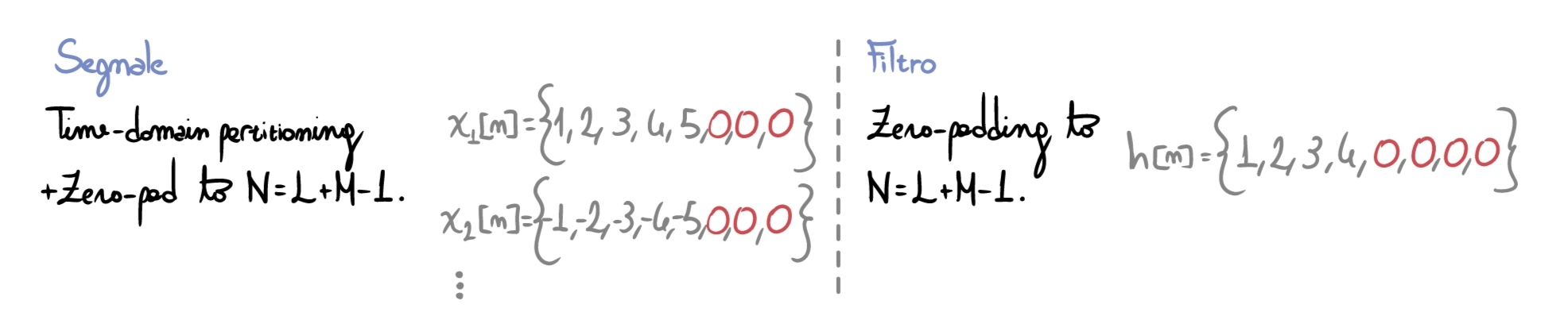
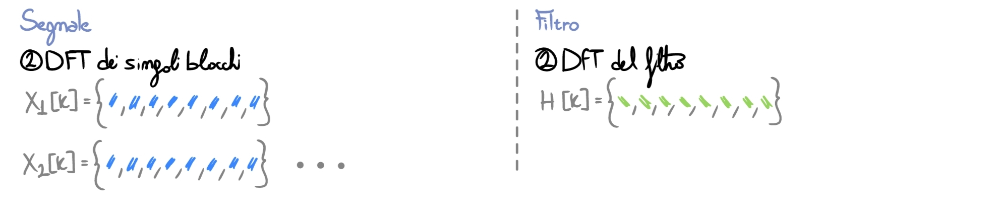
Once the filter and the frame have the same time length \(N\), we can move to the frequency domain by performing the FFT on the individual frames (note: in the images, I indicate the results of the various stages with symbols and colors: to understand the algorithm it is not necessary to know the sample values, it is enough to understand the processing flow).
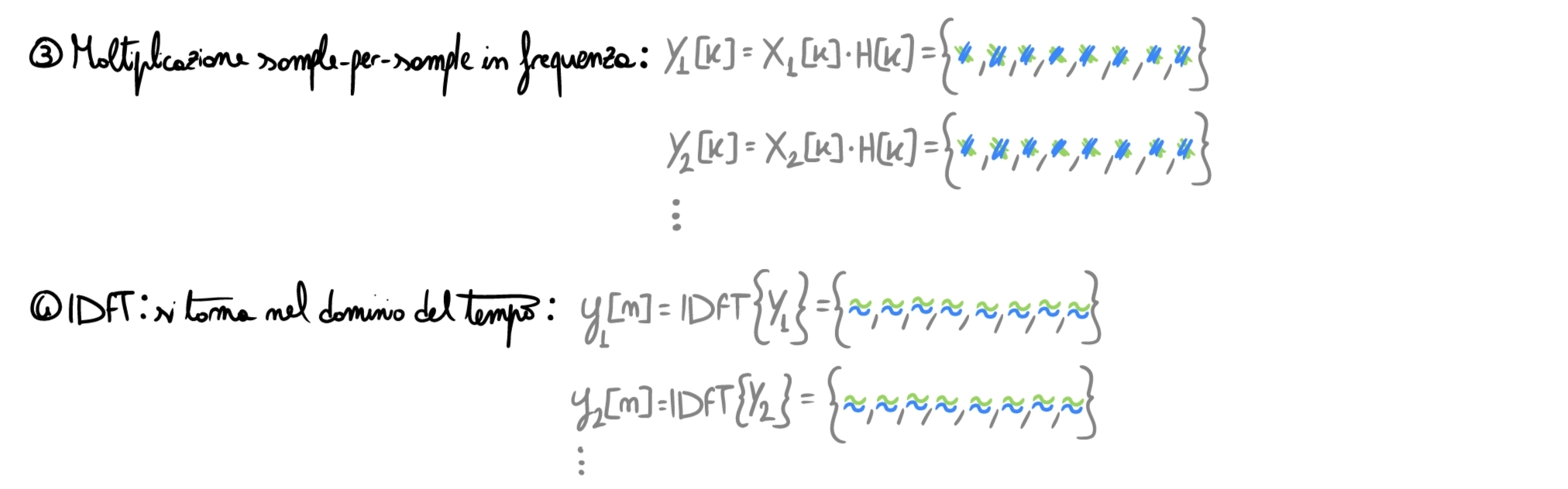
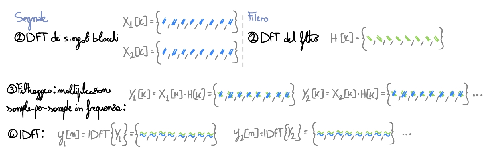
Now we perform the actual filtering: convolving in time equals multiplying sample by sample in frequency. Once finished, we go back to the time domain via IDFT.
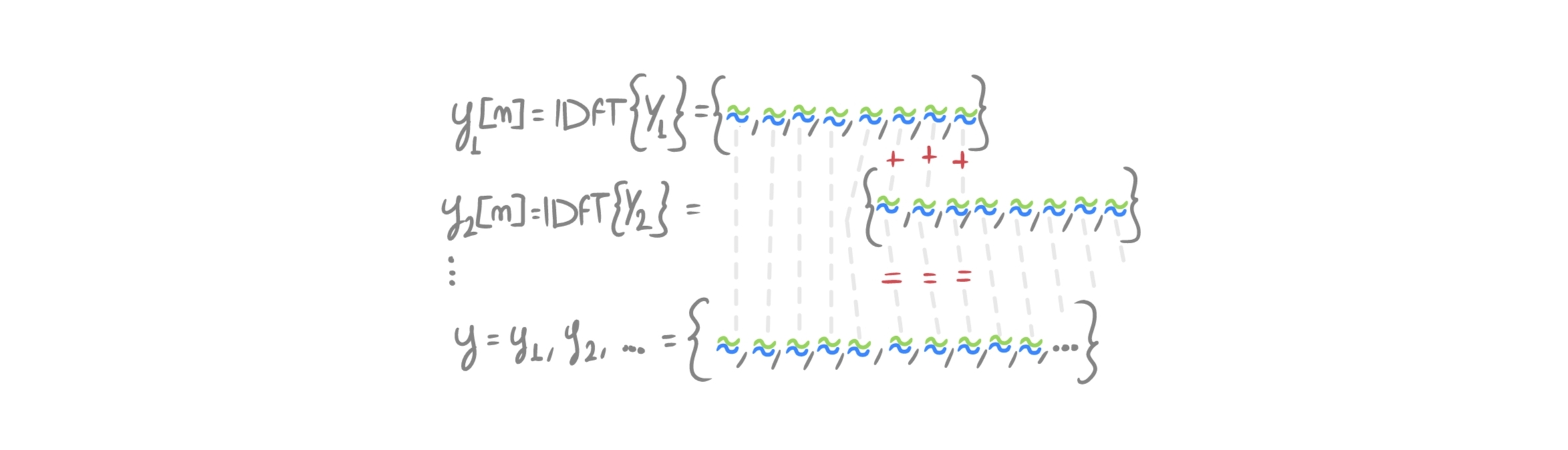
Now we reach the crucial moment: we must join the frames together and understand why we padded at the beginning.
Let’s compare with a “standard” convolution: processed signal length \(= 10\) samples, filter length \(=4\) samples, so the output signal will be \(L=10+4-1=13\) samples long.
If we put the computed frames \(y_i[n]\) one after another, we would obtain a signal of length \(16\): something is wrong.
The fact is that the padding done at the beginning is meant to contain the wrap around effect: as seen in the article on convolution, assuming that a signal is discrete in frequency means considering it periodic in the time domain (the signal/frame repeats infinitely). The convolution performed through the DFT is therefore circular, and zero-padding is precisely used to contain the tail of the convolution that, otherwise, would corrupt the initial samples. The information of the last \(M-1\) samples of the frame at \(t=n-1\) must therefore be added to the first \(M-1\) samples of the following frame \(t=n\), in order to reconstruct the entire output of what would be a linear convolution. In practice, the frames are overlapped like this:
Not convinced by the result? Let’s try a simple example, by hand, in the time domain.
Considering the signal \(x[n]=\{1,2,3,2\}\) and the filter \(h[n]=\{2,1,4,2\}\), let’s start with the preliminary operations needed for the computation:
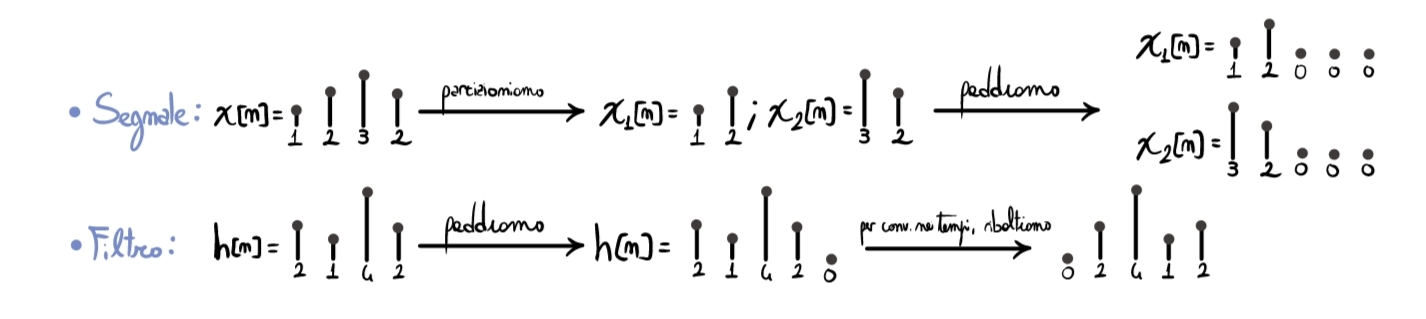
Now we can carry out the rest of the calculations:
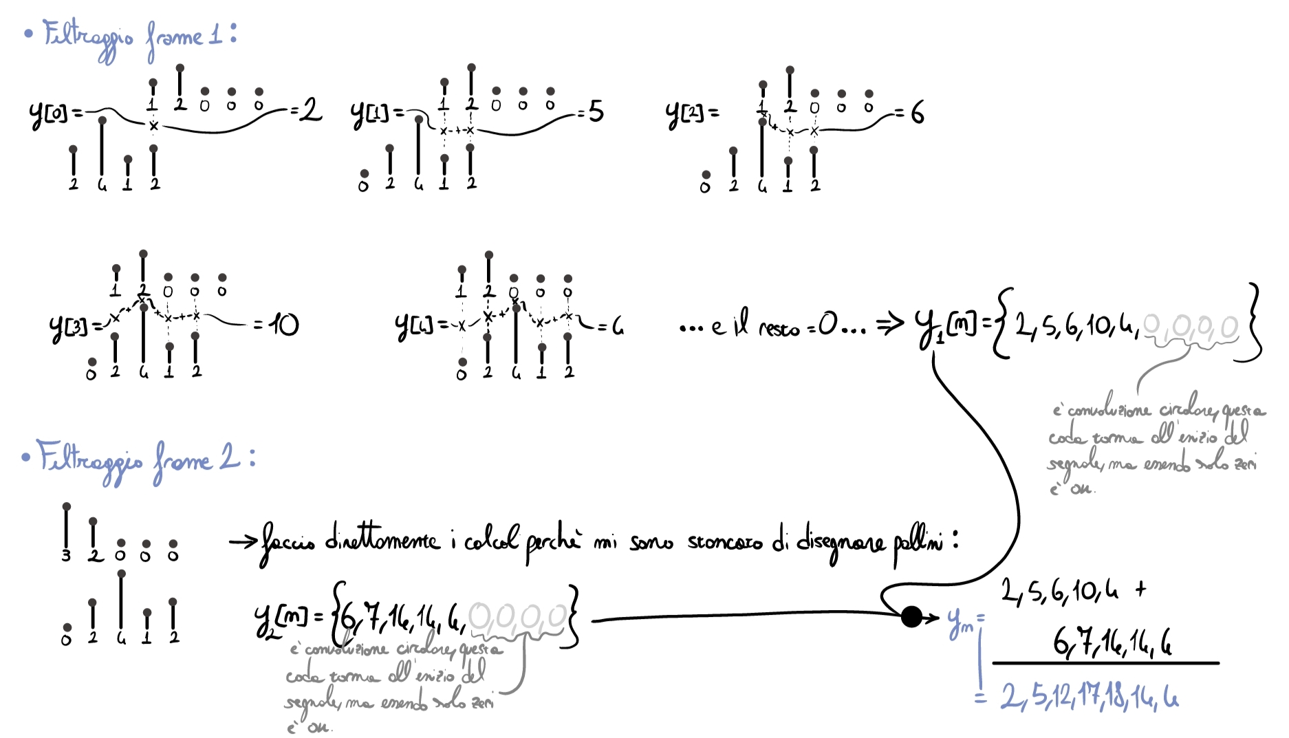
By performing a simple linear convolution, we would obtain the same result.
OverLap and Save (OLS)
It is a technique very similar to the previous one, but in the final step, instead of overlapping and summing, part of the output samples is discarded because they are corrupted by circular convolution. Let’s also analyze this algorithm step by step.
Consider the same example as in the previous OLA case:
- Filter of length \(M=4\) samples;
- Signal equal to \(x[n]=\{1,2,3,4,5,-1,-2,-3,-4,-5\}\);
- Partitions of the signal of length \(L=5\) samples.
- Convolution output (filter \(*\) signal partition) equal to \(N>=L+M-1\) samples. We again choose the frame length \(N=8\).
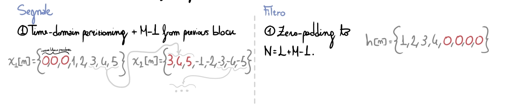
The first step consists of:
- padding the current signal frame with the last \(M-1\) samples of the previous frame;
- applying zero-padding to the filter as already seen before.
Then we move to the frequency domain, filter, and go back to the time domain as already seen:
We now reach the key step of the algorithm: we must understand how to put the various output pieces back together. During the first step we “extended” each frame by gluing the \(M-1\) samples of the previous frame to the left: this allowed us to
- “carry along” the information from past samples that still affects the samples of the current input block;
- use the first \(M-1\) samples as “containers” for the wrap-around phenomenon.
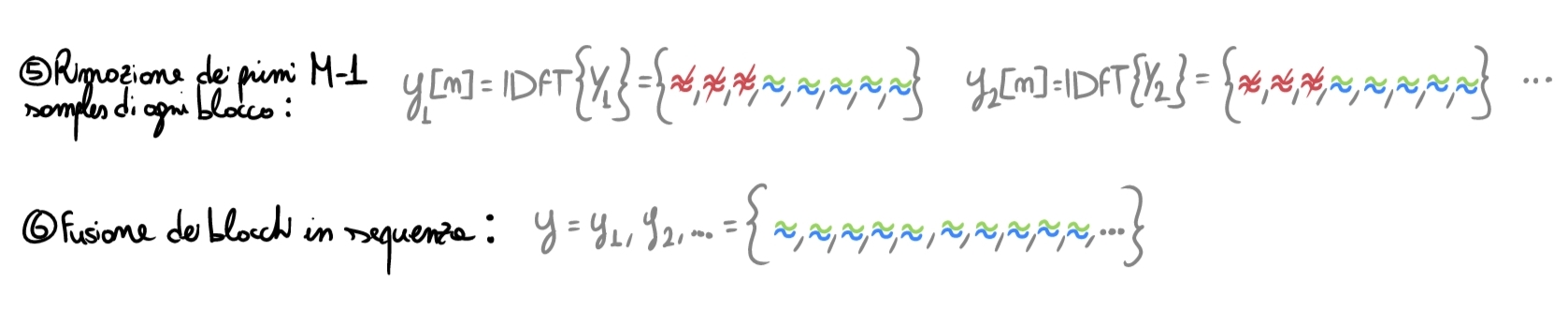
For this reason, now we simply discard those \(M-1\) initial samples corrupted by the tail of the circular convolution and merge the resulting frames back together:
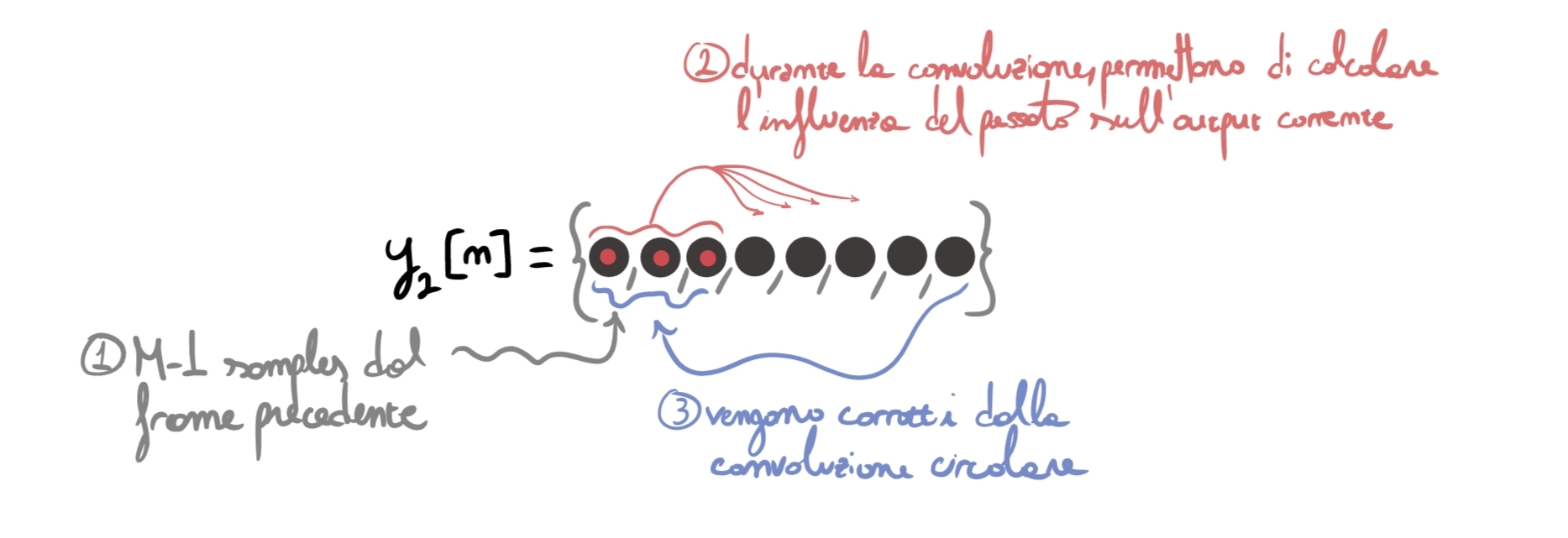
For additional clarity, I tried to graphically represent why it is necessary to add past samples at the beginning of each frame. The numbers (1,2,3) represent the temporal order in which events happen during convolution.
Partitioned Convolution
In the algorithms above, we used a very short filter. Now imagine the case where we want to convolve the input signal with a very long Impulse Response, beyond \(16{,}000\) samples. Partitioning the audio signal is not enough: for each frame we would have to pad up to \(N=L+M-1=\) more than \(16k\) samples, then perform, in real time, the FFT of this gigantic frame, multiply sample by sample, and then return to time. A huge workload that would generate a lot of latency.
So how do we solve this? We also partition the filter and perform the smallest possible number of operations in real time.
1. Offline operations
We perform all the operations that do not need to be executed in real time, to reduce the system load as much as possible at the crucial moment of execution.
First of all, we prepare the filter. We choose the partition length \(P\) (for both signal and filter partitions) and partition the filter into \(K=L/P\) partitions, where \(L\) is the length of the full filter. We pad each partition up to the length of the bins of our FFT (greater than the length of the convolution output, that is \(P_{signal}+P_{filter}-1=2P-1\)): let’s assume \(2P\).
Once we have the \(K\) partitions, we perform the FFT for each of them so that we already have these partial results ready for the real-time computation.
Let’s also prepare some structures we will need later:
- a buffer of length \(2P\) that will form our frame, whose first half of cells is initialized with zeros;
- a queue called FDL = Frequency Delay Line, which will be used to store past frames (in frequency) to compute their impact on the current output (we will see later).
2. Real-time operations
Ok, we are live. The guitarist turns on the pedal and starts playing on their Stratocaster. Samples start flowing from the cable into our pedal, and we start accumulating them in the buffer:
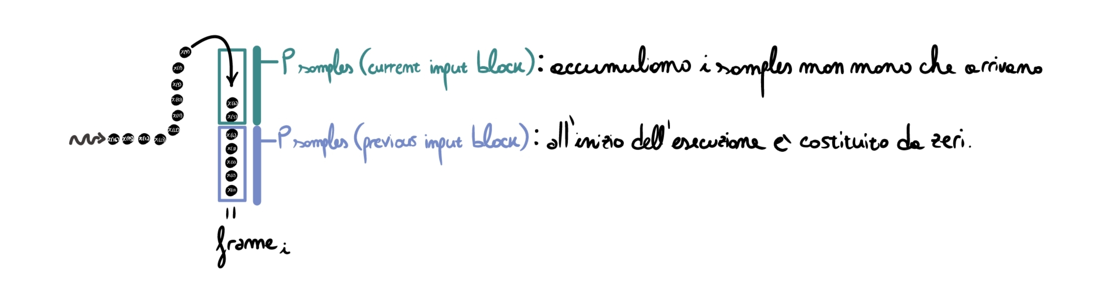
Note: the first \(P\) samples are:
- \(0\) if we are processing the first audio block (since there were no previous audio blocks);
- the last \(P\) samples of the previous frame if we are processing any frame other than the first. It is essentially the same step we saw in the OLS algorithm.
Once the frame reception is complete, we compute its FFT \(X_i[k]=FFT\{frame_i\}\) and store it in the FDL:
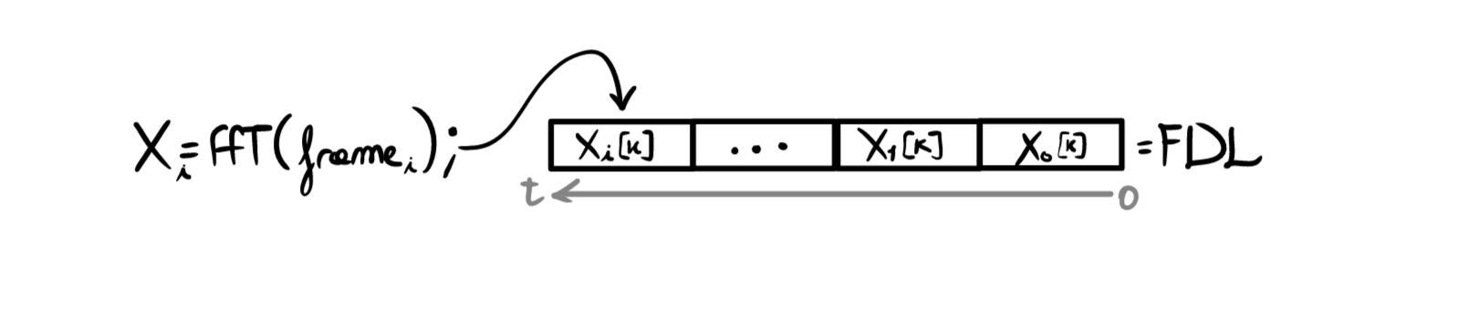
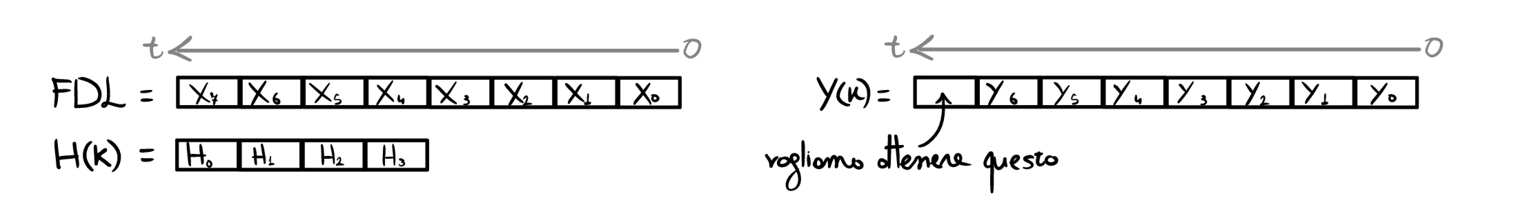
At this point we have FDL \(= \{X_0[k], X_1[k], ... ,X_i[k]\}\) representing our input, \(H=\{H_0[k], H_1[k],...H_K[k]\}\) representing the filter, and we want to obtain the current output frame \(Y_i[k]\).
To make understanding easier, consider the specific case with \(K=4\), where at a certain instant \(t\) we have already output \(6\) frames and we must process the seventh input frame (with the previous steps already completed).
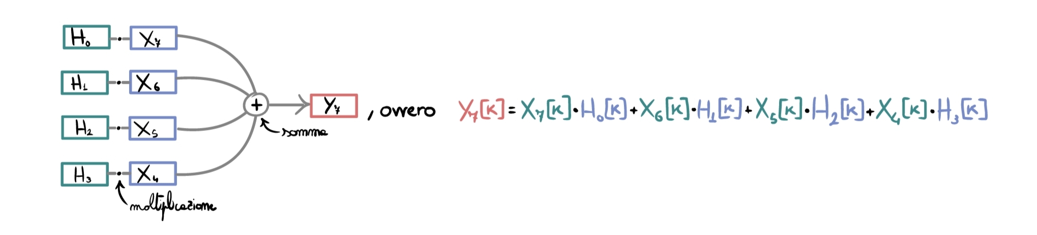
To apply the partitioned filter we must “recompose the convolution in time”, therefore “convolve the most recent signal frames with the initial parts of the IR, while previous signal frames with later IR blocks” (if you think about it, it is exactly what would happen if we did not partition the convolution):
The most complex part is over; from here on we proceed like a simple OLS:
- We perform the \(IFFT\) of the frame, returning to the time domain;
- We remove the first \(P\) samples (similarly to what we saw in the OLS algorithm);
- We output the remaining samples (that is, we reconstruct the output by placing frames one after another).
(It would also have been possible to implement the same algorithm using OLA).
The question that might arise now is: ok, but what are we saving? We are still using the entire filter, what would have changed compared to performing convolution with a simple OLS or OLA?
The answer lies in the percentage of operations we can precompute offline and those we are forced to perform in real time:
- in the case of OLS/OLA we can precompute zero-padding and the FFT of the filter, but we still must perform padding (up to \(N=L*M-1\)) plus FFT (of a frame of length \(N\), which, if \(M\) is very long, becomes very costly), the sample-by-sample multiplications in frequency, and then the return to time with overlap or discarding of the “transition samples” between frames.
- in the case of partitioned convolution we can not only precompute the filter partitions as above, but we can also use much shorter frames since \(P\) is not constrained below by the length of the full filter (for example, if the filter is \(16k\) samples long, with OLA we must use frames of length \(16k + L_{\text{signal part.}}-1\), while with partitioned convolution we are not constrained by the \(16k\) length of the filter because we can partition it into much smaller blocks). This means that the FFTs we must perform in real time are very short, because the rest of the frequency frames have been saved in the FDL, and the only thing left to do is multiply sample by sample in frequency and then return to time.
In practice, there is much less computational load in terms of FFT and IFFT per single block, thus drastically lowering output latency if the filter is very long.