Toolbox for studying DSP

We can view a signal as an object (a function) that carries information. The Polish guy at Starbucks who, at this exact moment, is yelling words I cannot understand, trying to tell me the coffee is ready, is attempting to transmit information (the coffee is ready) through a signal (yelling).

If we imagine that the Starbucks guy is a nightingale and is singing a single note to me, we could represent his yelling as a sinusoid at fixed frequency \(x(t)=A*cos(2*\pi*t+\phi)\), where \(A\) is the amplitude (how intense the yelling is), \(t\) is time, and \(\phi\) is the phase (we will talk about it shortly).

The function is nothing but a mapping between the amplitude levels taken by the signal and time \(t\). If this mapping is continuous in time, and therefore there are samples for every infinitesimal instant of time, then the signal is continuous (any sound we can perceive); otherwise, it is discrete.

Phase is a slightly more complex concept to understand: if we consider a signal \(x(t)=cos(2*\pi*t)\), it has phase \(\phi=0\) and, since \(cos(0)=1\), it will be \(1\) at \(t=0\). But if we add a phase, for example \(\phi=-\frac{\pi}{2}\), then we obtain the signal \(x'(t)=cos(2*\pi*t-\frac{\pi}{2})\), which is the same as saying \(x'(t)=cos(2*\pi*(t-\frac{1}{4})\). It is easy to see how \(t-\frac{1}{4}\) indicates a delay applied to the signal. So, phase represents an advance/delay applied to the signal, a translation on the time axis.

Forming a mental image of the phase of a single sinusoid is fairly simple, but the situation becomes problematic when we have to analyze more complex signals. In that case, as we will see later, dear Fourier will help us: we can assume that any signal can be decomposed into the sum of (an infinite number of) simple sinusoids, each with its own amplitude and its own phase. In that case, it is possible to obtain an understandable picture of the signal’s characteristics by transforming it to frequency and drawing magnitude and phase diagrams. Didn’t understand anything? It’s fine, we will explain it in detail later.

Let’s start from the very, very basics

Before starting the actual discussion, let’s review a few concepts that we surely already know, but that time may have made blurry in our minds.

Numbers

Numbers have been trusted companions of us hairless apes for a very, very long time. They came to our rescue as our society evolved and the things to keep track of (literally) increased. Let’s try to outline a brief timeline.

Natural numbers: they are simply the positive integers (1, 2, 3, 4, …) and we have used them since the beginning of civilization. For example, there are Babylonian and Egyptian warehouse tablets where inventory was tracked.
Integers: this is basically the set of natural numbers plus the negative ones (that is \(..., -3, -2, -1, 0, 1, 2, 3, ...\)). Even though they may feel intuitive to us people of the 21st century, the concept of a negative number was for a long time difficult to grasp (an amount smaller than nothing): if, as said, naturals have been used since the earliest civilizations (so more than 5000 years ago), negative numbers appear in mathematical texts only many centuries later, formalized in India around the 7th century AD and accepted in Europe even later.
Rational numbers: these too, used since the first civilizations, were born to manage the division of property and land. Concretely, they are fractional numbers such as \(\frac{5}{4}\), \(\frac{1}{2}\), and any other fraction with integer numerator and denominator (and \(\text{den}\neq 0\)).
Irrational numbers: you are a Greek mathematician living in Calabria, in Crotone, in the 5th century BC. There is no ‘Ndrangheta yet, so you decide to join the Pythagoreans. You live happily in your world of rational numbers (called that precisely for this reason) and everything is perfect, tied together by simple relationships between quantities (fractions with integer numerator and denominator and \(\text{den}\neq 0\)). One day, your friend Hippasus of Metapontum asks you to compute how long the diagonal of a square of side 1 is. You always knew he was a strange guy, but you decide to indulge him anyway. If we consider half of the square bounded by the diagonal and two sides, what we get is a right triangle. So the solution is very easy (and self-referential, for a Pythagorean): the Pythagorean theorem! Ok, so \(\text{diag}^2=\text{side}^2+\text{side}^2\), and therefore \(1^2+1^2=2\): the solution is \(\text{diag}=\sqrt{2}\). Wait, but what kind of number is \(\sqrt{2}\)? Can I express it as a fraction? It must be possible, since reality is made only of relationships between quantities, right? As they will discover, unfortunately not. And here appears a new species of numbers: irrationals. For centuries, mathematicians “procrastinated” in giving a rigorous definition of this class, using rather geometric workarounds to reach the same results.
Real numbers: by putting together rational and irrational numbers we obtain the real numbers, which we can imagine as all points on a continuous line. In practice they have been used, implicitly, for millennia, but a rigorous definition of this set arrives only in the 19th century, with the work of mathematicians such as Dedekind and Cantor.
Complex numbers: mathematics moved forward and often, in calculations, one would end up dealing with roots of negative numbers (e.g., the solution of \(x^2+1=0\)). For centuries, scientists treated these values as “imaginary” numbers (a name that then stuck), useful for computations but “not really existing”. Between the 16th and 17th centuries, in trying to solve equations of degree higher than two, mathematicians such as Cardano and Bombelli began using them systematically; in the 18th century Euler handled them very naturally, and between the late 18th and early 19th centuries, with Argand and Gauss, people stopped thinking of these numbers as a “trick” and treated them as a real mathematical and geometric object.

To have a clearer idea of the relationships between the above sets, here is a diagram taken from Wikipedia:

Numbers

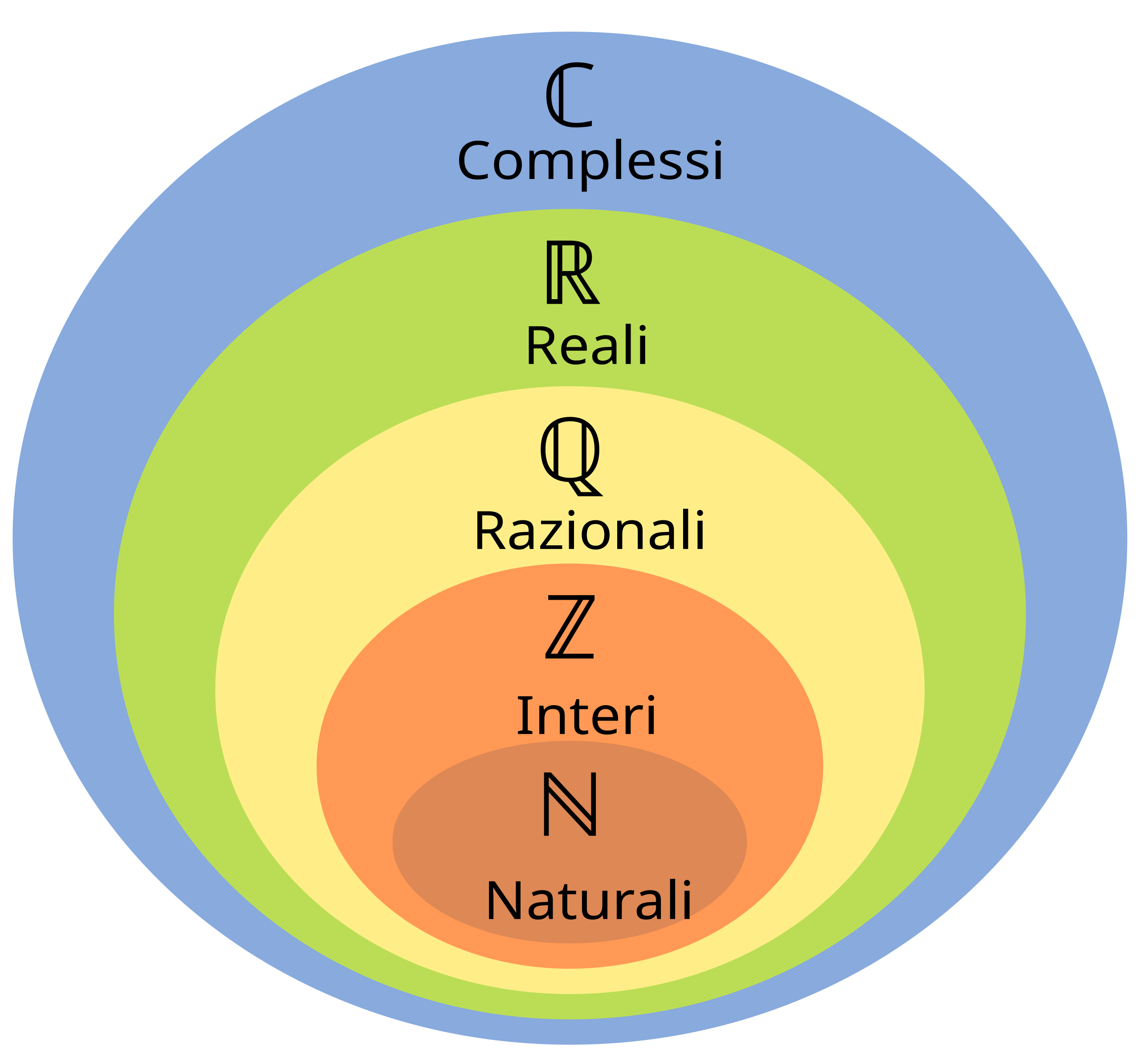
Assuming the reader is familiar with natural, real, rational, and irrational numbers, I will only write a short review of imaginaries.

Imaginary and complex numbers

The real numbers represented in the diagram above have a major structural limitation: they do not allow us to compute roots of negative numbers, such as \(\sqrt{-1}\). To fix this, we define an imaginary unit \(i=\sqrt{-1}\). This is the fundamental brick of imaginary numbers: any number \(b*i\) with \(b\in\mathbb{R}\) is a (purely) imaginary number.

We then define the set of complex numbers as the one containing numbers of the form \(a + b * i\), with \(a\in\mathbb{R}\) and \(b*i\in \mathbb{I}\).

These numbers are represented on a Cartesian graph called the “Argand-Gauss diagram”, where the real part is placed on the \(x\) axis and the imaginary part on the \(y\) axis, obtaining a point on the plane from these coordinates.

Gauss plane

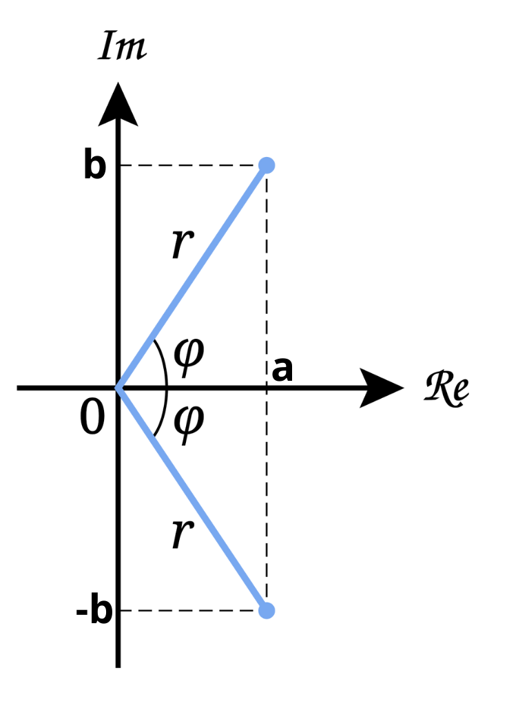
The segment that joins the origin to the point is called the magnitude and it is computed as \(r=\sqrt{a^2+b^2}\). The angle \(\theta\) in the picture is the phase, and it can be obtained from the relation \(b/a=\tan{\theta}\).

It is possible to represent the same complex number in different notations:

Algebraic form: the one seen above, where the number is written as the sum of its real and imaginary parts (\(c=a+b*i\) where \(a,b\in\mathbb{R}\) and \(i=\) the imaginary unit).
Trigonometric form: by computing the magnitude and phase of the complex number \(c\) from the previous point using the formulas \(r=\sqrt{a^2+b^2}\) and \(\theta=tan(b/a)\), we can represent the same quantity as \(c=r*[cos(\theta)+i*sin(\theta)]\). Of course, it is always possible to go back to the algebraic form using \(a=r*cos(\theta)\) and \(b=i*sin(\theta)\).
Exponential form: using \(\theta, r\) computed above, it is possible to express \(c\) through the so-called “exponential” form: \(c=r*e^{\theta*i}\).

Each of the forms above has specific use cases in which it is more convenient than the others.

Some important definitions that we will meet again later are:

Complex conjugate: given a number \(c=a+b*i\), the number \(c^*=a-b*i\) is its complex conjugate (imaginary part with opposite sign).
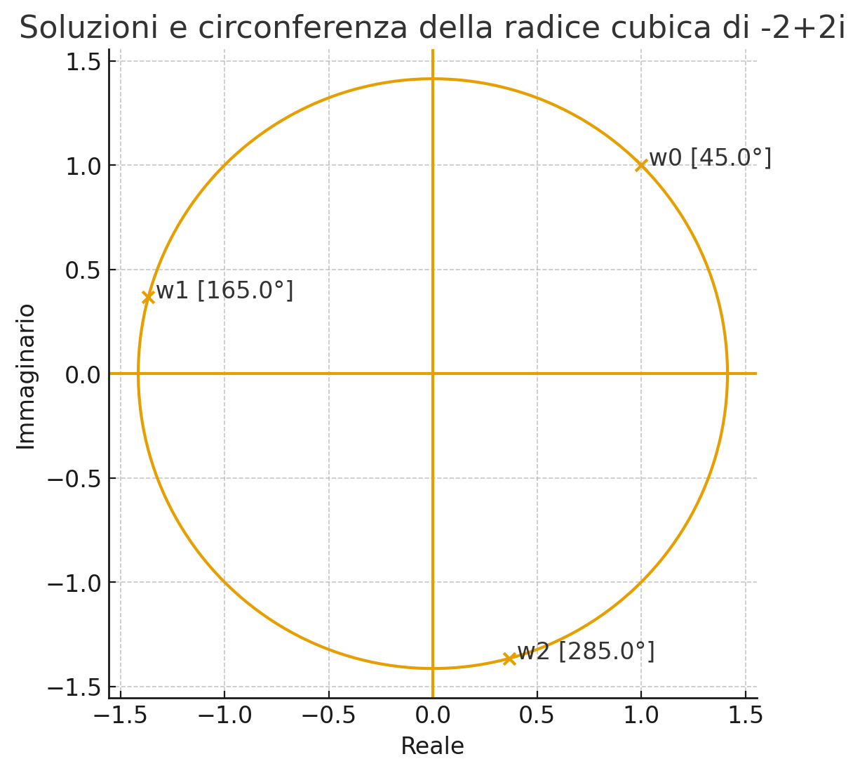
\(n\)-th roots: in the complex field, an \(n\)-th root has exactly \(n\) solutions. To understand the concept, let’s make an example. Consider the number \(c=-2+2i\) and write it in exponential form (\(\theta=tan(b/a)\) and \(r=\sqrt{a^2+b^2}\)). Let’s aim to compute the root \(\sqrt{c}^3=c^{1/3}\). The equation becomes \(c^{1/3}=r^{1/3}*e^{\frac{\theta}{3}*i}\) and, substituting the numerical values, \(c^{1/3}=8^{1/6}*e^{\frac{135^\circ}{3}*i}\), and therefore \(\sqrt{c}^3=\sqrt{2}*e^{45^\circ*i}\). This is only one of the \(n=3\) solutions. Considering the circle on the Gauss plane, the other two will be found with periodicity \(P=\frac{2\pi}{n}\) which in this case is \(P=\frac{2\pi}{3}=120^\circ\). We can visualize what we have said in the image below:

n-th roots

Trigonometry

It will be useful to recall some old and annoying trigonometry formulas:

\(sin(a ± b) = sin(a)* cos(b) ± cos(a)* sin(b)\);
\(cos(a ± b) = cos(a) *cos(b) ∓ sin (a)*sin(b)\);
\(sin(2t) = 2 sin(t) *cos(t)\);
\(cos(2t) = cos^2(t) − sin^2(t)\);
\(sin^2(t) = \frac{1 − cos(2t)}{2}\);
\(cos²t = \frac{1 + cos(2t)}{2}\).

Sequences

A sequence is a discrete function that associates a number to each index \(n\). For example, the sequence \(a_n=\frac{1}{n}\) with \(n=1,2,3,...\) consists of the values \(1,\frac{1}{2},\frac{1}{3},...\).

A very important concept is the limit of a sequence: saying that \(\lim_{n\to\infty} a_n = L\) means that, as the index n increases, the sequence values resemble \(L\) more and more.

From the concept of limit comes that of convergence of a sequence: if a sequence tends to a specific finite value, then it is said to converge to that value. There are some notable cases to remember:

Geometric sequence: it is of the form \(a_n=r^n\). Such a sequence:
- converges to \(0\) if \(\|r\|<1\);
- converges to \(1\) if \(r=1\);
- is indeterminate if \(r<-1\);
- diverges in magnitude if \(r \le -1\).
Polynomial sequence: it is of the form \(a_n=n^p\). In that case, the sequence diverges if \(p>0\).

There are also “dominance relationships” between these sequences: if we multiply a geometric by an exponential, the resulting sequence follows the exponential trend, since the exponential grows/decays faster than the geometric.

Series

Starting from sequences we can define series as the infinite sum of all terms of a sequence: \(S_N=\sum_{n=n_0}^{N} a_n\). A series is said to converge if \(\lim_{N\to\infty} S_N = S\), with \(S\) finite. If that limit does not exist or is infinite, then the series diverges.

Given a series \(\sum a_n\), we then distinguish two types of convergence:

Absolute convergence if the series \(\sum_{n=n_0}^{\infty} \|a_n\| < \infty\) converges (in practice, the series of the absolute value of the sequence \(a_n\) converges);
Conditional convergence: if the series \(\sum_{n=n_0}^{\infty} a_n < \infty\) converges, but the series \(\sum_{n=n_0}^{\infty} \|a_n\| < \infty\) diverges. In that case convergence is weaker (e.g., the series with term \(a_n=\frac{-1^n}{n}\) converges, but the one with term \(\|a_n\|=\frac{1^n}{n}\) diverges).

Ok, but how do we practically understand whether a series converges or not? It is not always easy, but we can rely on some tricks:

A necessary condition (but not sufficient) for a series to converge is that the sequence it contains converges to 0. So if we encounter a series whose sequence does not go to 0, we should not even waste time: it diverges.
Comparison with a known series: imagine we have two series \(\sum{a_n}\) and \(\sum{b_n}\). We already know \(\sum{a_n}\) and we know it converges. We want to understand whether \(\sum{b_n}\) behaves the same, but we do not know how. Well, if we are lucky enough to have \(\sum{b_n}<\sum{a_n}\), then we can immediately conclude that \(\sum{b_n}\) also converges.
Asymptotic comparison: given two series \(\sum{a_n}\) and \(\sum{b_n}\), both \(>0\), if \(\lim_{n\to\infty}\frac{a_n}{b_n}=c\), with \(0<c<\infty\), then either both converge or both diverge. Of course, the goal is to use a known series which, when put in ratio with the other in this context, yields a finite limit, so we can conclude the other series has the same behavior as the known one.
Ratio test: given a series \(\sum{a_n}\), by computing the ratio \(L=\lim_{n\to\infty}\left\|\frac{a_{n+1}}{a_n}\right\|\) we have:
- if \(L<1\) it converges absolutely;
- if \(L=1\) we cannot draw any conclusion from this test;
- if \(L>1\) the series diverges.
Root test: similar to the previous one, this test tells us that given a series \(\sum{a_n}\), by computing \(L=\limsup_{n\to\infty}\sqrt[n]{\|a_n\|}\) we can deduce that
- if \(L<1\) the series converges absolutely;
- if \(L=1\) we cannot draw conclusions;
- if \(L>1\) the series diverges.
Alternating series test: given an alternating-sign series, writable in the form \(\sum{(-1)^n*a_n}\), we can use this convergence criterion. The test states that if \(a_n\) is \(>=0\), monotonically decreasing, and tending to \(0\), then the overall series converges.

All very nice. But how do we use these “comparison criteria” if we do not know any known series? The doubt is legitimate, and indeed there are many “known” series whose behavior is known. I will not write a detailed explanation because this is not the main topic of the text, but for our purposes it is important to know the geometric series, which will be very useful later.

In practice, the geometric series is \(\sum_{n=0}^{\infty} r^n\) and it converges if and only if the following conditions are both satisfied:

\(\|r\|<1\);
\(\sum_{n=0}^{\infty} r^n = \frac{1}{1-r}\).

Example on series and sequences

Consider the series \(\sum_{n=0}^{\infty} (-1)^n r^n\). For which \(r\) does it converge? Let’s first analyze the case \(r>0\).

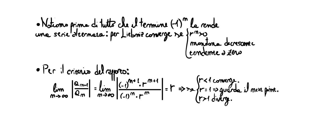
Noting that \(r^n\) is a geometric sequence, we can deduce that it tends to \(0\) only for \(\|r< 1\|\), while for values \(=1\) it converges to 1. We therefore deduce that the “right constraint” of the convergence set is \(r< 1\). Let’s see what happens on the left:

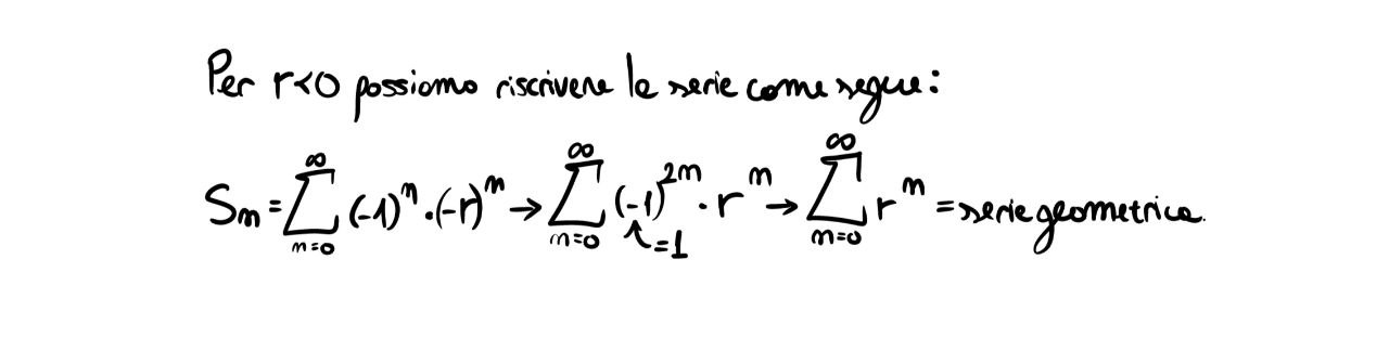
As already seen, the series above converges for \(\|r\|< 1\).

In summary, we deduce that the series converges for values \(r \in (-1,1)\), excluding the endpoints.

To be continued …

I will not go deeper into the topics above, even though they were treated very superficially and incompletely, because this was only a brief review in preparation for understanding the article on convolution.

Angelo Antona, 3 DECEMBER 2025